Voltage stability margin and P-V curves: how many MW can a bus take?
A load flow tells you whether a network works today. It does not tell you how far it is from the point where it stops working. A P-V curve does: it plots the voltage at a bus against the load as the load is increased, up to the last point where a load flow still has a solution. The distance from today’s load to that point, in MW, is the voltage stability margin.
The question behind it is usually practical. A data center, an electrolyser or a factory wants to connect, and somebody has to say how many MW the bus can take and what stops it from taking more.
What a P-V curve looks like
At light load the voltage falls slowly as the load grows. The more power the network has to carry, the more reactive power its lines and transformers absorb, and the faster the voltage drops. At some load the curve turns vertical. This is the tip, or nose, of the curve: beyond it there is no operating point, and in a real system the voltage collapses.
For the simplest case, a stiff source feeding a load through a reactance X, the tip can be written down. At unity power factor the largest power that can be delivered is
Pmax = V2 / 2X
and the voltage at the load there is about 0.71 p.u. Two things follow from this. A network normally leaves its allowed voltage band long before it reaches the tip. And a lagging power factor moves the tip to the left: the same two-bus network that delivers 151 MW at unity power factor delivers about 110 MW at a power factor of 0.95.
Three limits, and the first one counts
On the way to the tip a network meets three limits. The first one it meets is the real limit of the connection.
- Voltage limit. The load at which the first bus drops below the minimum voltage, typically 0.95 p.u.
- First overload. The load at which the first line or transformer passes 100 % loading.
- Voltage collapse. The tip of the curve, where the load flow no longer solves.
Reporting only the collapse point gives a number that looks generous and cannot be used. Reporting only the voltage limit hides how steep the curve is behind it. You need all three.
Worked example: a new load on the IEEE 39-bus system
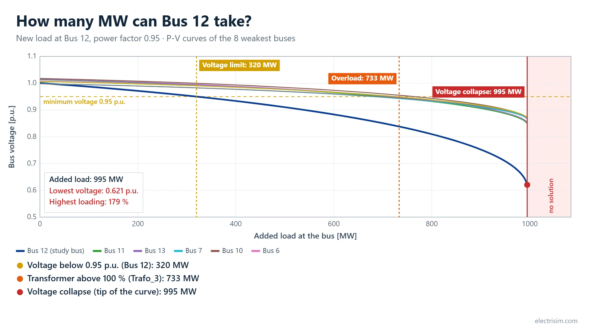
The chart at the top of this page is the result for a new load with a power factor of 0.95 at Bus 12 of the IEEE 39-bus system, which is one of the diagram templates in Electrisim.
| Limit | New load at Bus 12 | What sets it |
|---|---|---|
| Voltage limit (0.95 p.u.) | 320 MW | The first bus leaves the voltage band |
| First overload (100 %) | 733 MW | A transformer reaches its rating |
| Voltage collapse | 995 MW | The load flow has no solution beyond this |
So Bus 12 can take about 320 MW as the network stands. Reactive compensation at the bus would lift the voltage limit towards the 733 MW where a transformer becomes the constraint. The collapse point at 995 MW is three times the usable figure, which is why it should never be quoted alone.
Which bus has the most room?
The same study can be repeated for every bus. Electrisim adds the load at one bus, finds its limits, removes it and moves on to the next one. On the IEEE 39-bus system the answer runs from 965 MW at Bus 32 down to 318 MW at Bus 12, so Bus 12 is the weakest place in this network to connect a large load.
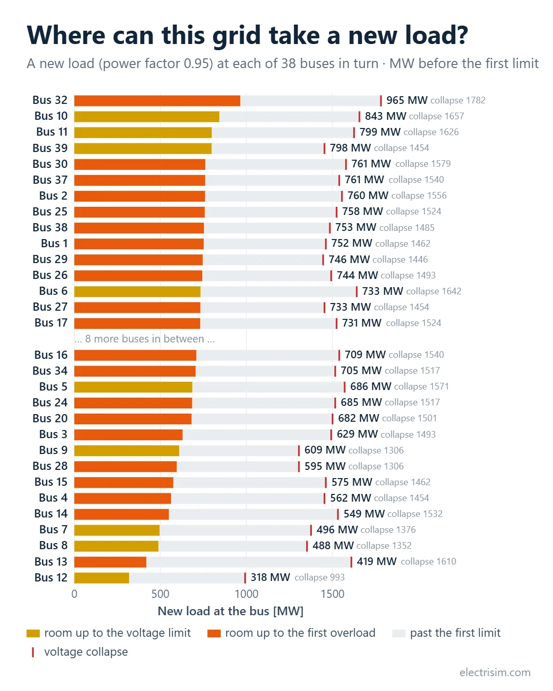
Each bus is studied on its own. The ranking does not say what happens when loads are added at two buses at once.
How to run it in Electrisim
- Run a normal load flow first, so you know the network solves as drawn.
- Optional: select the bus you are interested in on the diagram. Select several buses to compare only those.
- Click Simulate → Voltage Stability Margin (P-V Curves).
- Choose how the load grows: all loads together, a new load at one bus, or a comparison of buses.
- Set the minimum voltage, the maximum loading and 50 or 60 Hz, then click Calculate.
The results window gives the three margins in MW, the P-V chart for the eight buses with the lowest voltage at the tip, and a table of the 20 weakest buses. The chart can be saved as an image or exported as a video, and every point of the curves can be downloaded as CSV. The study needs a subscription and runs on pandapower. All parameters are described in the voltage stability documentation.
How the tip is found
Electrisim raises the load with a step that doubles each time until a load flow fails, then halves the interval between the last solved and the first failed value until it is within 0.2 %. Each load flow starts from the previous solution, which keeps it on the upper, stable branch of the curve. On the two-bus network above the result is 151.2 MW against the textbook 151.25 MW, and 109.5 MW against 109.50 MW at a power factor of 0.95.
What the numbers assume
- The extra power comes from the slack bus (the External Grid or the slack generator). Other generators keep their set points.
- Generator reactive limits apply only where they are entered in the model.
- The network is intact. With an outage the margins are lower, so check the important ones with N-1 contingency analysis.
- This is steady-state voltage stability. It is not a dynamic simulation; for that, see transient stability.
The IEEE 39-bus system is under New diagram in the app, so the example above can be repeated as it is: app.electrisim.com.
Related: Data center interconnection study, power factor correction calculator and the glossary.